Adjust modules

These modules offer the basic tools for global adjustments of the image being processed. All operations are pixel-wise.

Brightness

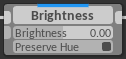
Brightness:Modifies image brightness Preserve Hue:Preserves input image hue in LCH space Group:Adjust Color Space:LRGB

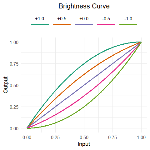
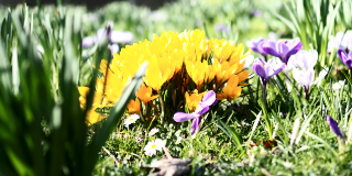
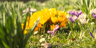
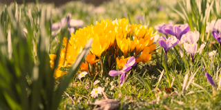
This module changes the brightness of the image by adjusting the slope at \(0.0\) with the Brightness parameter, and preserves the white point by compressing the curve toward \(1.0\) (1). The Preserve Hue parameter applies the hue of the input image to that of the output image in LCH space (2).

Warning

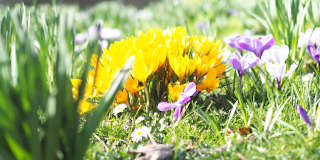
The module is intended to preserve the brightened image’s black point and white point. However, color channels might be pushed out of gamut when Preserve Hue is enabled.

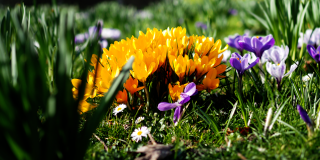
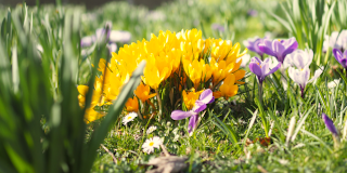
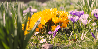
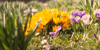
Brightness	Preserve Hue: On	Preserve Hue: Off
-1.0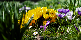
+0.0
+1.0

(1)\[\begin{split}\begin{align} B & = Brightness + 1 \\ Output_{RGB} & = (1-B) \cdot Input_{RGB}^2 + B \cdot Input_{RGB} \end{align}\end{split}\]

(2)\[Output_H = Input_H\]

---

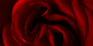
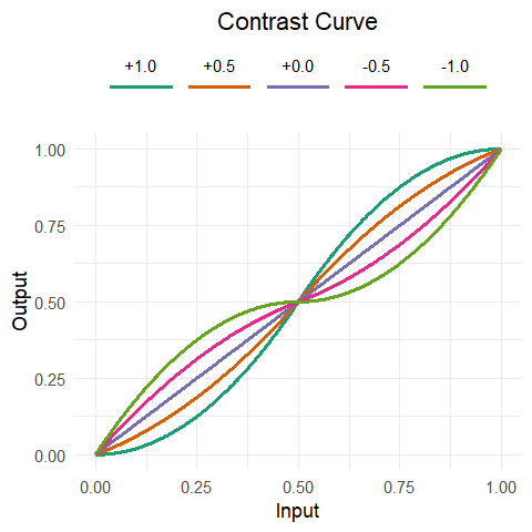
Contrast

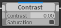
Contrast:Modifies image mid-tone contrast Saturation:Preserves image saturation instead of chroma Group:Adjust Color Space:LAB

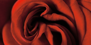
This module changes the contrast of the image by adjusting the LAB lightness slope at \(0.5\) with the Contrast parameter, and preserves the black point and white point by compressing the extremes (3). The Saturation parameter enables scaling of the chroma channel to preserve constant saturation instead of constant chroma when the lightness channel is modified (3).

This module does not account for changes in saturation perception due to a change in scene luminance contrast, as this is very much scene-dependent. A perceived decrease in saturation when increasing contrast and vice versa is observable. This can be corrected appropriately with the Vibrance or Saturation module.

Warning

The luminance black point and white point are preserved. Color channels may be pushed out of gamut.

Note

Setting the Contrast parameter to \(0.0\) creates a contrast curve with a slope of \(0.0\) in the mid-tones. This results in a very flat output image.

Contrast	Saturation: On	Saturation: Off
-1.0
+0.0
+1.0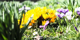

Contrast	Saturation: On	Saturation: Off
-1.0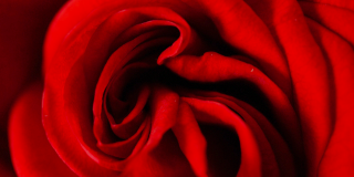
+0.0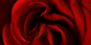
+1.0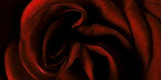

(3)\[\begin{split}\begin{align} C &= Contrast + 1 \\ I &= 2 \cdot Input_L - 1 \\ O &= \left\{ \begin{array}{rl} (C-1) \cdot I^2 + I \cdot C & I < 0 \\ (1-C) \cdot I^2 + I \cdot C & I > 0 \end{array} \right. \\ Output_L &= \frac{O + 1}{2} \\ \end{align}\end{split}\]

(4)\[Output_{AB} = Input_{AB} \cdot (Output_L - Input_L)\]

---

Vibrance

Vibrance:Increases color saturation, mainly in less saturated areas Group:Adjust Color Space:LCH

This module changes the color saturation such that less saturated colors are boosted. It adjusts the LCH chroma channel slope at \(0.0\) with the Vibrance parameter, and preserves the saturation point by compressing the curve toward \(1.0\) (5). The Vibrance effect is modulated with the image’s lightness channel, such that the effect decreases linearly for darker colors. In addition, the output image lightness is decreased proportional to the increase in chroma \(\times 0.2\) to further enhance color perception.

Warning

While chroma in the LCH space is limited to \(1.0\), the resulting colors at this limit are still outside the sRGB gamut. This module does not necessarily prevent oversaturation.

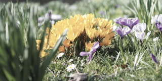
Value	Vibrance	Saturation \(\times 0.5\)
-1.0
+0.0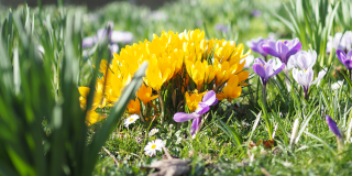
+1.0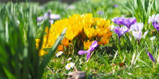

(5)\[\begin{split}\begin{align} V &= Vibrance \cdot Input_L + 1 \\ Output_C &= (1-V) \cdot Input_C^2 + V \cdot Input_C \\ Output_L &= Input_L \cdot (1 - 0.2 \cdot (Output_C - Input_C)) \end{align}\end{split}\]

Note

The chroma curve for the Vibrance module is equivalent to the Brightness module curve. However, the strength of the Vibrance parameter is in addition modulated by the input image lightness, making the curve dependent on both lightness and chroma.

---

Saturation

Saturation:Increases color saturation linearly Group:Adjust Color Space:LCH

This module changes the LCH chroma linearly with the Saturation parameter as multiplication factor (6). It allows for full desaturation of the input image, as well as unbounded oversaturation.

Value	Saturation
-1.0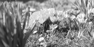
-0.5
+0.0
+0.5
+1.0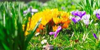

(6)\[Output_C = Input_C \cdot Saturation\]

---

Temperature

Temperature:Source correlated color temperature (K) Tint:Green tint Group:Adjust Color Space:XYZ

This module corrects color cast due to the difference in scene illuminants compared to the white point of the viewing environment. The Temperature parameter indicates the correlated color temperature of the illuminant of the scene. The source color temperature is converted to a source white reference \(RefSource_{LMS}\) (8). The Tint parameter additionally scales the source white reference Y to correct a green cast. The destination white reference \(RefDest_{LMS}\) is computed for \(T = 6500\,K\) illuminant to match the D65 standard illuminant of sRGB. Chromatic adaptation is performed using the Von Kries transform in LMS space (9). A Bradford matrix (7) is used for the conversion from XYZ to LMS.

Note

The conversion from correlated color temperature to chromaticity is performed using the daylight locus as reference instead of the black body locus. This should be more appropriate for naturally occurring light.

Temperature	Tint: 0.9	Tint: 1.0	Tint: 1.1
3800 K
4700K
5600K
6500K
8300K
11000K
15500K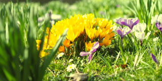

(7)\[\begin{split}M_{Bradford} = \left[ \begin{array}{rrr} 0.8951 & 0.2664 & 0.1614 \\ -0.7502 & 1.7135 & 0.0367 \\ 0.0389 & 0.0685 & 1.0296 \end{array} \right]\end{split}\]

(8)\[\begin{split}\begin{align} T &= Temperature \\ x &= \left\{\begin{array}{rl} \frac{0.27475E9}{T^3} - \frac{0.98598E6}{T^2} + \frac{1.17444E3}{T} + 0.145986 & T < 4000 \\ \frac{-4.6070E9}{T^3} + \frac{2.9678E6}{T^2} + \frac{0.09911E3}{T} + 0.244063 & 4000 < T < 7000 \\ \frac{-2.0064E9}{T^3} + \frac{1.9018E6}{T^2} + \frac{0.24748E3}{T} + 0.237040 & 7000 < T \end{array}\right. \\ y &= -3 \cdot x^2 + 2.87 \cdot x - 0.275 \\ \left[ \begin{array}{c} L \\ M \\ S \end{array} \right] &= M \cdot \left[ \begin{array}{c} X \\ Y \\ Z \end{array} \right] = M \cdot \left[ \begin{array}{c} \frac{x}{y} \\ Tint \\ \frac{1-x-y}{y} \end{array} \right] \end{align}\end{split}\]

(9)\[\begin{split}Output_{XYZ} = M^{-1} \cdot \left[ \begin{array}{ccc} \frac{RefDest_L}{RefSource_L} & 0 & 0 \\ 0 & \frac{RefDest_M}{RefSource_M} & 0 \\ 0 & 0 & \frac{RefDest_S}{RefSource_S} \end{array} \right] \cdot M \cdot Input_{XYZ}\end{split}\]

---

Curve Modules

The curve modules allow fine control of image adjustments. They define a mapping between one parameter and another specified as a user-defined function. The output of the mapping function can either set an absolute value, or offset or modulate the original value.

---

Parametric Curve

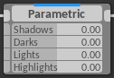
Shadows:Adjustment of the shadows Darks:Adjustment of the dark tones Lights:Adjustment of the light tones Highlights:Adjustment of the highlights Group:Adjust > Curves Color Space:LAB

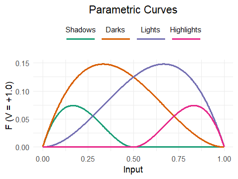
This module adjusts the lightness L in four tonal regions. The overall adjustment is a brightness offset factor \(F_{Tone}\) for each region (10), where \(V_{Tone}\) is one of the Shadows, Darks, Lights, or Highlights parameters. These curves are scaled and linearly modulated depending on the tonal range. They are combined in (11), where \(F_{Shadows}\) and \(F_{Highlights}\) are modulated with the headroom remaining after \(F_{Darks} + F_{Lights}\) is applied. The saturation is preserved in the AB components (12).

Tone	-1.0	+1.0
Shadows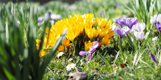
Darks
Lights
Highlights

(10)\[\begin{split}\begin{align} I &= Input_L \\ F_{Shadows} &= \left\{\begin{array}{rl} V_{Shadows} \cdot I \cdot (2 \cdot I - 1)^2 & I<0.5 \\ 0 & I>0.5 \end{array}\right. \\ F_{Darks} &= V_{Darks} \cdot (I - 1)^2 \cdot I \\ F_{Lights} &= -V_{Lights} \cdot (I - 1) \cdot I^2 \\ F_{Highlights} &= \left\{\begin{array}{rl} 0 & I<0.5 \\ - V_{Highlights} \cdot (I-1) \cdot (2 \cdot I - 1)^2 & I>0.5 \end{array}\right. \end{align}\end{split}\]

(11)\[\begin{split}\begin{align} O &= Input_L + F_{Darks} + F_{Lights} \\ Output_L &= O + F_{Shadows} \cdot \frac{O}{Input_L} + F_{Highlights} \cdot \frac{1-O}{1-Input_L} \end{align}\end{split}\]

(12)\[Output_{AB} = Input_{AB} \cdot (Output_L - Input_L)\]

---

Curve L

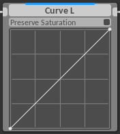
Preserve Saturation:  Maintain constant saturation Group:Adjust > Curves Color Space:LAB

This module sets the output lightness L as function of the input lightness. The implementation is similar to that of the Contrast module (13), but with a user-defined curve \(f\). The Saturation parameter enables scaling of the chroma channel to preserve constant saturation instead of constant chroma when the lightness channel is modified (14).

(13)\[Output_L = f(Input_L)\]

(14)\[Output_{AB} = Input_{AB} \cdot (Output_L - Input_L)\]

---

Curve Y

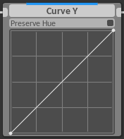
Preserve Hue:Preserves input image hue in LCH space Group:Adjust > Curves Color Space:XYZ

This module sets the output luminance Y as function of the input luminance. The implementation is similar to that of the Brightness module (15), but with a user-defined curve \(f\). The Preserve Hue parameter applies the hue of the input image to that of the output image in LCH space (16).

(15)\[Output_Y = f(Input_Y)\]

(16)\[Output_H = Input_H\]

---

Advanced Curve modules

Group:Adjust > Curves > Advanced Color Space:LCH

These curves map one component of the LCH color space against another in the following way, where \(f\) is the curve function:

Curve L-L:\(Output_L = f(Input_L)\) Curve L-C:\(Output_C = Input_C \cdot f(Input_L)\) Curve L-H:\(Output_H = Input_H + f(Input_L)\)

---

Curve C-L:\(Output_L = Input_L \cdot f(Input_C)\) Curve C-C:\(Output_C = f(Input_C)\) Curve C-H:\(Output_H = Input_H + f(Input_C)\)

---

Curve H-L:\(Output_L = Input_L \cdot ((f(Input_H)-1) \cdot Input_C + 1)\) Curve H-C:\(Output_C = Input_C \cdot f(Input_H)\) Curve H-H:\(Output_H = Input_H + f(Input_H)\)

Note

The H-L curve effect is modulated with chroma, such that low chroma input with noisy hue does not result in noisy lightness in the output.

---

Mask Curve Modules

Group:Adjust > Curves > Advanced Color Space:LCH > Y

These curves create a single-channel mask output based on curve \(f\) applied to the input channel:

Select L:\(Output_Y = f(Input_L)\) Select C:\(Output_Y = f(Input_C)\) Select H:\(Output_Y = f(Input_H)\)